NGSolve Examples

In this example we will have a look on how we can solve a multiphysics problem in NGSolve and the NGSPy interface. Therefore, we will consider a fluid-structure interaction problem, where the Navier-Stokes equations for the fluid part

$$\rho \frac{\partial u}{\partial t}+\rho (u\cdot \mathrm{\nabla })u-\rho \nu \mathrm{\Delta }u+\mathrm{\nabla }p=f$$ $$\text{div}(u)=0$$

and the elastic wave equation for the elastic part

$$\rho \frac{{\partial }^{2}d}{\partial t^2}-\text{div}(F\mathrm{\Sigma })=g$$

are used.

The Navier-Stokes equations are given in Eulerian form, whereas the elasticity problem is formulated in Lagrangian coordinates. Thus, to couple these two equations we use the Arbitrary Lagrangian Eulerian form (short ALE) for the fluid part.

We will work always on a fixed reference domain. Therefore, we will transform the Navier-Stokes equations back to it. Let $\mathrm{\Phi }(x,t)=\text{id}+d$ describe the movement of the mesh, where $d$ is the displacement. Then we define $$u\circ \mathrm{\Phi }=\hat{u}$$ and use the chain rule $${\mathrm{\nabla }}_{x}u\circ \mathrm{\Phi }={\mathrm{\nabla }}_{\hat{x}}\hat{u}{F}^{-1},$$

where $F=\mathrm{\nabla }\mathrm{\Phi }$ denotes the deformation gradient. Next, we take the time derivative and get $$\frac{\partial u}{\partial t}\circ \mathrm{\Phi }=\frac{\partial \hat{u}}{\partial t}-{\mathrm{\nabla }}_{\hat{x}}\hat{u}{F}^{-1}\frac{\partial \mathrm{\Phi }}{\partial t}=\frac{\partial \hat{u}}{\partial t}-{\mathrm{\nabla }}_{\hat{x}}\hat{u}{F}^{-1}\dot{d}.$$

The time derivative of the deformation $\dot{d}$ is called the mesh velocity and describes the relative movement of the mesh. Next we apply the transformation theorem where we get the determinant of the deformation gradient $J=det(F)$ and with this the equations in weak form read

$${\int }_{{\mathrm{\Omega }}^f}J(\rho \frac{\partial \hat{u}}{\partial t}\cdot \hat{v}+\rho ((\hat{u}-\dot{d})\cdot \mathrm{\nabla })\hat{u}{F}^{-1}\cdot \hat{v}+\rho \nu \mathrm{\nabla }\hat{u}{F}^{-1}:\mathrm{\nabla }\hat{v}{F}^{-1}-\text{tr}(\mathrm{\nabla }\hat{v}{F}^{-1})p)dx=0\mathrm{\forall }v,$$ $${\int }_{{\mathrm{\Omega }}^f}J\text{tr}(\mathrm{\nabla }\hat{u}{F}^{-1})qdx=0\mathrm{\forall }q.$$

The elastic wave equation does not have to be transformed. We rewrite it as a system of first order equations in time and the variational formulation is

$${\int }_{{\mathrm{\Omega }}^s}\frac{\partial d}{\partial t}\cdot vdx={\int }_{{\mathrm{\Omega }}^s}u\cdot vdx\mathrm{\forall }v,$$

$${\int }_{{\mathrm{\Omega }}^s}\rho \frac{\partial u}{\partial t}\cdot w+(F\mathrm{\Sigma }):\mathrm{\nabla }wdx=0\mathrm{\forall }w.$$

Beneath the displacement $d$, the velocity $u$ and the deformation gradient $F=I+\mathrm{\nabla }d$ the material law $\mathrm{\Sigma }$ has to be considered. We will use the material law of Hook. With the Cauchy-Green strain tensor $C=F^{T}F$ and the Green strain tensor $E=\frac{1}{2}(C-I)$ the law reads $$\mathrm{\Sigma }=2\mu E+\lambda \text{tr}(E)I,$$ where $\mu$ and $\lambda$ are two material parameters.

The interface conditions for fluid-structure interaction have also to be considered before we can couple the equations. The velocity and displacement have to be continuous over the interface and the forces from the fluid and the solid have to be in equilibrium $${\int }_{{\mathrm{\Gamma }}_I}{\sigma }^{s}nds={\int }_{{\mathrm{\Gamma }}_I}{\sigma }^{f}nds.$$

As we are using a monolithic approach, where both equations are solved together in each time step, this equation is always fulfilled as a natural condition in weak sense. Therefore, we add both, the Navier-Stokes and the elastic wave equation, and then simply neglect the two force terms.

The last important ingredient is the deformation extension. The mesh velocity $\dot{d}$ in the Navier-Stokes equations is artificial and has to be constructed from the given dispacement of the solid on the interface. A very simple approach would be to solve a Poisson problem on the fluid domain with the solid displacement as dirichlet boundary conditions on the interface and homogeneuos dirichlet conditions on the other boundaries. This works only for small deformations as the triangles get pressed through others. Thus, we will penalize the volume compression on the one hand and play around with a space dependent function to manipulate the stiffness of the problem, which yields an elasticity problem with the material law of Neo-Hook $$N=h(x)\mu (\text{tr}(E)+\frac{2\mu }{\lambda }det(C{)}^{-\frac{\lambda }{2\mu }}-1),$$

where $h(x)$ denotes the space dependent function. The extension can have a negative effect on the elastic wave equations on the solid domain. Therefore, we multiply it with a small parameter to minimize this effect.

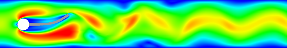
As an example we will consider the following benchmark propsed by Turek and Hron. It is based on the classical flow around cylinder benchmark, where additionally an elastic flag is "glued" behind the obsticle.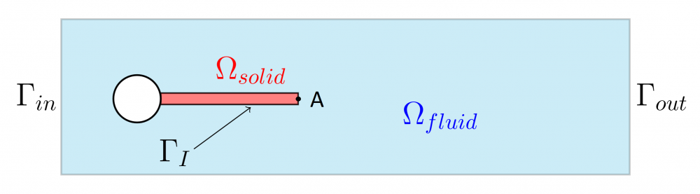

The geometry can be constructed easily with splines,

def GenerateMesh(order, maxh=0.12, L=2.5, H=0.41):
    r = 0.05
    D = 0.1
    
    geom = SplineGeometry()
    pnts = [ (0,0), (L,0), (L,H), (0,H), (0.2,0.15), (0.240824829046386,0.15), (0.248989794855664,0.19), (0.25,0.2), (0.248989794855664,0.21), (0.240824829046386,0.25), (0.2,0.25), (0.15,0.25), (0.15,0.2), (0.15,0.15), (0.6,0.19), (0.6,0.21), (0.55,0.19), (0.56,0.15), (0.6,0.15), (0.65,0.15), (0.65,0.2),(0.65,0.25), (0.6,0.25), (0.56,0.25), (0.55,0.21), (0.65,0.25),(0.65,0.15) ]
    pind = [ geom.AppendPoint(*pnt) for pnt in pnts ]

    geom.Append(['line',pind[0],pind[1]],leftdomain=1,rightdomain=0,bc="wall")
    geom.Append(['line',pind[1],pind[2]],leftdomain=1,rightdomain=0,bc="outlet")
    geom.Append(['line',pind[2],pind[3]],leftdomain=1,rightdomain=0,bc="wall")
    geom.Append(['line',pind[3],pind[0]],leftdomain=1,rightdomain=0,bc="inlet")

    geom.Append(['spline3',pind[4],pind[5],pind[6]],leftdomain=0,rightdomain=1,bc="circ")
    geom.Append(['spline3',pind[6],pind[7],pind[8]],leftdomain=0,rightdomain=2,bc="circ2")
    geom.Append(['spline3',pind[8],pind[9],pind[10]],leftdomain=0,rightdomain=1,bc="circ")
    geom.Append(['spline3',pind[10],pind[11],pind[12]],leftdomain=0,rightdomain=1,bc="circ")
    geom.Append(['spline3',pind[12],pind[13],pind[4]],leftdomain=0,rightdomain=1,bc="circ")

    geom.Append(['line',pind[6],pind[14]],leftdomain=2,rightdomain=1,bc="interface")
    geom.Append(['line',pind[14],pind[15]],leftdomain=2,rightdomain=1,bc="interface")
    geom.Append(['line',pind[15],pind[8]],leftdomain=2,rightdomain=1,bc="interface")


    geom.SetMaterial(1, "fluid")
    geom.SetMaterial(2, "solid")
    
    mesh = Mesh(geom.GenerateMesh(maxh=maxh))
    mesh.Curve(order)
    
    return mesh

where the boundaries are identified with strings, and also the domains have names.

For the spatial discretization we will use the Taylor-Hood elements for the Navier-Stokes equations and also H1-conforming elements for the elastic wave equation. Thus, we can use one global space for the velocity and the displacement.

V = VectorH1( mesh, order = order, dirichlet = "inlet|wall|circ|circ2" )
Q = H1( mesh, order = order - 1, definedon = "fluid" )
D = VectorH1( mesh, order = order, dirichlet = "inlet|wall|outlet|circ|circ2" )

With the definedon flag, we can tell the pressure space, that it lives only on the fluid domain.

Before we come to the bilinearforms, we define the following functions.

def SolidBFI(term, **args):
    return SymbolicBFI(term.Compile(), definedon=mesh.Materials("solid"), **args)
def FluidBFI(term, **args):
    return SymbolicBFI(term.Compile(), definedon=mesh.Materials("fluid"), **args)

With the definedon flag, we can tell the bilinearform, that it is only defined on one domain, either on the fluid or on the solid domain.

For the time discretization we will use the Crank-Nicolson method $${\int }_{t^n}^{t^{n+1}}f(s)ds\approx \frac{\tau }{2}(f(t^{n+1})+f(t^n)).$$ The Navier-Stokes equations in ALE description discretized in space and time are given as:

# M du/dt
a += FluidBFI( 0.5*rhof/tau*InnerProduct(J*(u-velocityold), v)+0.5*rhof/tau*InnerProduct(Jold*(u-velocityold), v) )
# Laplace
a += FluidBFI( 0.5*rhof*nuf*InnerProduct(J*grad(u)*Finv, grad(v)*Finv)+0.5*rhof*nuf*InnerProduct(Jold*2*Sym(graduold*Finvold), (grad(v)*Finvold)) )
# Convection
a += FluidBFI( 0.5*rhof*InnerProduct(J*(grad(u)*Finv)*u, v)+0.5*rhof*InnerProduct(Jold*(graduold*Finvold)*velocityold, v) )
# mesh velocity
a += FluidBFI( -0.5*rhof/tau*InnerProduct((J*grad(u)*Finv)*(d-deformationold), v)-0.5*rhof/tau*InnerProduct((Jold*graduold*Finvold)*(d-deformationold), v) )
# Pressure/Constraint
a += FluidBFI( -J*(Trace(grad(v)*Finv)*p+Trace(grad(u)*Finv)*q)- 1e-9*p*q )

The elasticity problem is formulated with the following lines.

# M du/dt
a += SolidBFI( rhos/tau*InnerProduct(u-velocityold, v) )
# Material law
a += SolidBFI( 0.5*InnerProduct(2*F*Stress(E), grad(v))+0.5*InnerProduct(2*Fold*Stress(Eold), grad(v)) )
#dd/dt = u
a += SolidBFI( InnerProduct(u+velocityold-2.0/tau*(d-deformationold), w))

Next, we extend the deformation from the solid to the fluid domain.

factor = 1e-20*mus
def minCF(a,b) : return IfPos(a-b, b, a)
Vdist = H1(mesh, order=2)
gfdist = GridFunction(Vdist)
gfdist.Set( minCF( (x-0.6)*(x-0.6)+(y-0.19)*(y-0.19), (x-0.6)*(x-0.6)+(y-0.21)*(y-0.21) ) )

def NeoHookExt (C, mu=1,lam=1):
    return 0.5 * mu * (Trace(C-I) + 2*mu/lam * Pow(Det(C), -lam/2/mu) - 1)
a += SymbolicEnergy( (factor*(1/sqrt(gfdist*gfdist+1e-12)) * NeoHookExt(C)).Compile(), definedon=mesh.Materials("fluid"))

To increase the inflow velocity depending on time, we have to extend the new velocity into the domain, before solving the system. This can be done by solving a stokes problem with the new velocity as dirichlet data only on the fluid domain. To tell the solver on which domain it should work, we have to define the according degrees of freedom, which is done in terms of bitarrays.

bts = Y.FreeDofs() & ~Y.GetDofs(mesh.Materials("solid"))
bts &= ~Y.GetDofs(mesh.Boundaries("wall|inlet|circ|interface|circ2"))
invstoke = stokes.mat.Inverse(bts, inverse = inverse)

Now, we can use Newton's method to solve the arising system.

while t < tend-tau/2.0:
    #update velocity
    par.Set(Force(t)-Force(t-tau))
    tmp.components[0].Set( uinflow, BND, definedon=mesh.Boundaries("inlet") )
    rstokes.data = stokes.mat*tmp.vec
    tmp.vec.data -= invstoke*rstokes
    gfu.components[0].vec.data += tmp.components[0].vec
    gfu.components[1].vec.data += tmp.components[1].vec
        
    #Newton's method
    for it in range(10):
        a.Apply(gfu.vec, r.vec)
        a.AssembleLinearization(gfu.vec)
        inv = a.mat.Inverse(X.FreeDofs(), inverse=inverse)
                
        w.data = inv*r.vec    
        err = InnerProduct(w, r.vec)
                        
        gfu.vec.data -= w
                
        if abs(err) < 1e-20: break
            
    Redraw(blocking=True)
    gfuold.vec.data = gfu.vec