Using BBND to compute the magnetic field of a thin wire

Featured

Using BBND to compute the magnetic field of a thin wire

Christopher Lackner

The newly introduced BBND feature of Netgen/NGSolve allows us to compute the magnetic field of a thin wire by approximating it with operators on the 1D line segment. In this example we want to compute the field of the following coil geometry:

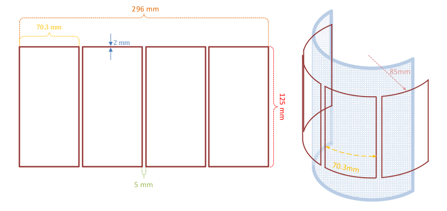
To see how this geometry is constructed using Netgen, have a look at BBND - A New Feature of Netgen 6.2, the file createCoil.py is attached again. This SplineGeometry is then added to a CSGeometry containing an enclosing Sphere.

geo = CSGeometry()
geo.Add(Sphere(Pnt(0,0,0),0.3).bc("outer").mat("air"))
surfaces = CreateCyl([0,0,0],[0,0,1],[0,0.085,0],0.073,0.125,0.01,4,0.005)
for surface in surfaces:
    geo.AddSplineSurface(surface)

mesh = Mesh(geo.GenerateMesh(maxh=0.05))
Draw(mesh)

This generates this (pretty raw) mesh:

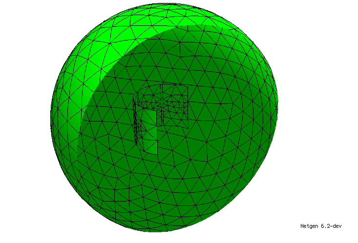
Note that one could change the meshsize at each surface and/or segment. On this geometry we want to solve the following problem:

Find $u \in H_{\text{curl}}(\Omega) $ such that $$ \int_{\Omega} \frac{1}{\mu} \text{ curl}(u) \text{ curl}(v) - k^2 \varepsilon u v \hspace{0.1cm} dx + \int_{\Gamma_W} \sigma d k i u_T v_T \hspace{0.1cm} dx - \int_{\partial \Omega} ik \sqrt{\frac{\varepsilon}{\mu}} u_T v_T \hspace{0.1cm} dx = \int_{\Gamma_C} I_s v_T \hspace{0.1cm} dx $$ for all $ v \in H_{\text{curl}}(\Omega) $. Here $\mu, \varepsilon $ and $\sigma$ are the usual electromagnetic coefficients, $d$ is the diameter of the wire, $i$ the imaginary unit, $k $ the frequency, $\Gamma_W$ the BBND lines defined as "wire", $\Gamma_C$ the BBND lines defined as "contact", $I_s$ the on the contact imposed current and $u_T$ and $v_T$ the respective traces depending on the codimension of the integral. The boundary term on $\partial \Omega$ is a first order transparent boundary condition, to approximate an open domain.

To implement this we define a HCurl finite element space and the corresponding TrialFunction and TestFunction

fes = HCurl(mesh,order=2,complex=True)
u,v = fes.TrialFunction(), fes.TestFunction()

After defining the coefficients (they are just constants in our example), we can define the left- and right hand side as BilinearForm and LinearForm.

a = BilinearForm(fes)
a += SymbolicBFI(1./mu * curl(u) * curl(v) - k*k*eps * u * v)
a += SymbolicBFI(sigma * d * k * 1J * u.Trace().Trace() * v.Trace().Trace(), definedon=mesh.BBoundaries("wire"))
a += SymbolicBFI(-1J * k * sqrt(eps/mu) * u.Trace() * v.Trace(), definedon=mesh.Boundaries("outer"))

f = LinearForm(fes)
f += SymbolicLFI(Is * v.Trace().Trace(), definedon=mesh.BBoundaries("contact"))

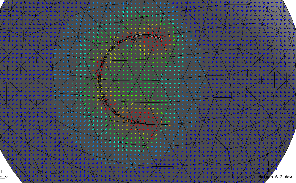
The second call to SymbolicBFI is interesting, we integrate here over the line segments defined as "wire" in our geometry. The function mesh.BBoundaries(...) returns this region. The function .Trace() returns the appropriate trace operator of the respective space, for the HCurl this is the tangential trace. Another call to .Trace() now gives the trace operator on the codimension 2 object.

After defining a GridFunction on the space we only have to assemble everything and solve the system. Then we can draw our solution and the magnetic field.

u = GridFunction(fes,"u")

with TaskManager():
    a.Assemble()
    f.Assemble()
    u.vec.data = a.mat.Inverse() * f.vec

Draw(u)
Draw(curl(u),mesh,"B")

If you have any questions feel free to leave a comment below!

NGSolve Examples

Using BBND to compute the magnetic field of a thin wire