7.1 Shape optimization via the shape derivative

In this tutorial we discuss the implementation of shape optimization algorithms to solve

\[\min_{\Omega} J(\Omega) := \int_{\Omega} f(x)\;dx, \quad f\in C^1(\mathbf{R}^d).\]

The analytic solution to this problem is

\[\Omega^*:= \{x\in \mathbf{R}^d:\; f(x)\le 0\}.\]

This problem is solved by fixing an initial guess \(\Omega_0\subset \mathbf{R}^d\) and then considering the problem

\[\min_{X} J((\mbox{id}+X)(\Omega_0)),\]

where \(X:\mathbf{R}^d \to \mathbf{R}^d\) are (at least) Lipschitz vector fields. We approximate \(X\) by a finite element function.

Initial geometry and shape function

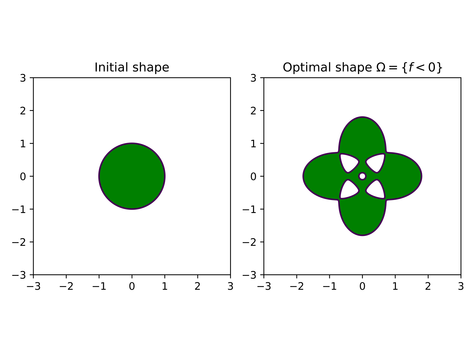
We choose \(f\) as

\[\begin{split}\begin{array}{rl} f(x,y) =& \left(\sqrt{(x - a)^2 + b y^2} - 1 \right) \left(\sqrt{(x + a)^2 + b y^2} - 1 \right) \\ & \left(\sqrt{b x^2 + (y - a)^2} - 1 \right) \left(\sqrt{b x^2 + (y + a)^2} - 1 \right) - \varepsilon. \end{array}\end{split}\]

where \(\varepsilon = 0.001, a = 4/5, b = 2\). The corresponding zero level sets of this function are as follows. The green area indicates where \(f\) is negative.

Let us set up the geometry.

# Generate the geometry
from ngsolve import *

# load Netgen/NGSolve and start the gui
from ngsolve.webgui import Draw
from netgen.geom2d import SplineGeometry

geo = SplineGeometry()
geo.AddCircle((0,0), r = 2.5)

ngmesh = geo.GenerateMesh(maxh = 0.08)
mesh = Mesh(ngmesh)
mesh.Curve(2)

#gfset.vec[:]=0
#gfset.Set((0.2*x,0))
#mesh.SetDeformation(gfset)
#scene = Draw(gfzero,mesh,"gfset", deformation = gfset)

# define the function f and its gradient
a =4.0/5.0
b = 2
f = CoefficientFunction((sqrt((x - a)**2 + b * y**2) - 1) \
                * (sqrt((x + a)**2 + b * y**2) - 1) \
                * (sqrt(b * x**2 + (y - a)**2) - 1) \
                * (sqrt(b * x**2 + (y + a)**2) - 1) - 0.001)

# gradient of f defined as vector valued coefficient function
grad_f = CoefficientFunction((f.Diff(x),f.Diff(y)))

# vector space for shape gradient
VEC = H1(mesh, order=1, dim=2)

# grid function for deformation field
gfset = GridFunction(VEC)
gfX = GridFunction(VEC)

Draw(gfset)

Shape derivative

\[DJ(\Omega)(X) = \int_\Omega f \mbox{div}(X) + \nabla f\cdot X\;dx\]

# Test and trial functions
PHI, PSI = VEC.TnT()

# shape derivative
dJOmega = LinearForm(VEC)
dJOmega += (div(PSI)*f + InnerProduct(grad_f, PSI) )*dx

Bilinear form

\[(\varphi,\psi) \mapsto b_\Omega(\varphi,\psi):= \int_\Omega (\nabla \varphi+\nabla \varphi^\top): \nabla\psi+\varphi\cdot \psi\; dx.\]

to compute the gradient \(X:= \mbox{grad}J(\Omega)\) by

\[b_\Omega(X,\psi) = DJ(\Omega)(\psi)\quad \text{ for all } \quad \psi \in H^1(\Omega)\]

# bilinear form for H1 shape gradient; aX represents b_\Omega
aX = BilinearForm(VEC)
aX += InnerProduct(grad(PHI) + grad(PHI).trans, grad(PSI)) * dx
aX += InnerProduct(PHI, PSI) * dx

The first optimisation step

Fix an initial domain \(\Omega_0\) and define

\[\mathcal J_{\Omega_0}(X):= J((\mbox{id} + X)(\Omega_0)).\]

Then we have the following relation between the derivative of \(\mathcal J_{\Omega_0}\) and the shape derivative of \(J\):

\[D\mathcal J_{\Omega_0}(X_n)(X) = DJ((\mbox{id}+X_n)(\Omega_0))(X\circ(\mbox{id}+X_n)^{-1}).\]

Here

• \((\mbox{id}+X_n)(\Omega_0)\) is current shape

Now we note that \(\varphi \mapsto \varphi\circ(\mbox{id}+X_n)^{-1}\) maps the finite element space on \((\mbox{id}+X_n)(\Omega_0)\) to the finite element space on \(\Omega_0\). Therefore the following are equivalent:

• assembling \(\varphi \mapsto D\mathcal J_{\Omega_0}(X_n)(\varphi)\) on the fixed domain \(\Omega_0\)

• assembling \(\varphi \mapsto DJ((\mbox{id}+X_n)(\Omega_0))(\varphi)\) on the deformed domain \((\mbox{id}+X_n)(\Omega_0)\).

# deform current domain with gfset
mesh.SetDeformation(gfset)

# assemble on deformed domain
aX.Assemble()
dJOmega.Assemble()

mesh.UnsetDeformation()
# unset deformation

Now let’s make one optimization step with step size \(\alpha_1>0\):

\[\Omega_1 = (\mbox{id} - \alpha_1 X_0)(\Omega_0).\]

# compute X_0
gfX.vec.data = aX.mat.Inverse(VEC.FreeDofs(), inverse="sparsecholesky") * dJOmega.vec

print("current cost ", Integrate(f*dx, mesh))
print("Gradient norm ", Norm(gfX.vec))

alpha = 20.0 / Norm(gfX.vec)

gfset.vec[:]=0
scene = Draw(gfset)
# input("A")
gfset.vec.data -= alpha * gfX.vec
mesh.SetDeformation(gfset)
#draw deformed shape
scene.Redraw()
# input("B")

print("cost after gradient step:", Integrate(f, mesh))
mesh.UnsetDeformation()
scene.Redraw()

Optimisation loop

Now we can set up an optimisation loop. In the second step we compute

\[\Omega_2 = (\mbox{id} - \alpha_0 X_0 - \alpha_1 X_1)(\Omega_0)\]

by the same procedure as above.

import time


iter_max = 50
gfset.vec[:] = 0
mesh.SetDeformation(gfset)
scene = Draw(gfset,mesh,"gfset")

converged = False

alpha =0.11#100.0 / Norm(gfX.vec)
# input("A")
for k in range(iter_max):
    mesh.SetDeformation(gfset)
    scene.Redraw()
    Jold = Integrate(f, mesh)
    print("cost at iteration ", k, ': ', Jold)

    # assemble bilinear form
    aX.Assemble()

    # assemble shape derivative
    dJOmega.Assemble()

    mesh.UnsetDeformation()

    gfX.vec.data = aX.mat.Inverse(VEC.FreeDofs(), inverse="sparsecholesky") * dJOmega.vec

    # step size control

    gfset_old = gfset.vec.CreateVector()
    gfset_old.data = gfset.vec

    Jnew = Jold + 1
    while Jnew > Jold:

        gfset.vec.data = gfset_old
        gfset.vec.data -= alpha * gfX.vec

        mesh.SetDeformation(gfset)

        Jnew = Integrate(f, mesh)

        mesh.UnsetDeformation()

        if Jnew > Jold:
            print("reducing step size")
            alpha = 0.9*alpha
        else:
            print("linesearch step accepted")
            alpha = alpha*1.5
            break

    print("step size: ", alpha, '\n')

    time.sleep(0.1)
    Jold = Jnew

Using SciPy optimize toolbox

We use the package scipy.optimize and wrap the shape functions around it.

We first setup the initial geometry as a circle of radius r = 2.5 (as before)

# The code in this cell is the same as in the example above.

from ngsolve import *
from ngsolve.webgui import Draw
from netgen.geom2d import SplineGeometry

import numpy as np

ngsglobals.msg_level = 1

geo = SplineGeometry()
geo.AddCircle((0,0), r = 2.5)

ngmesh = geo.GenerateMesh(maxh = 0.08)
mesh = Mesh(ngmesh)
mesh.Curve(2)

# define the function f

a =4.0/5.0
b = 2
f = CoefficientFunction((sqrt((x - a)**2 + b * y**2) - 1) \
                * (sqrt((x + a)**2 + b * y**2) - 1) \
                * (sqrt(b * x**2 + (y - a)**2) - 1) \
                * (sqrt(b * x**2 + (y + a)**2) - 1) - 0.001)

# Now we define the finite element space VEC in which we compute the shape gradient

# element order
order = 1

VEC = H1(mesh, order=order, dim=2)

# define test and trial functions
PHI = VEC.TrialFunction()
PSI = VEC.TestFunction()


# define grid function for deformation of mesh
gfset = GridFunction(VEC)
gfset.Set((0,0))

# only for new gui
#scene = Draw(gfset, mesh, "gfset")

#if scene:
#    scene.setDeformation(True)

# plot the mesh and visualise deformation
#Draw(gfset,mesh,"gfset")
#SetVisualization (deformation=True)

Shape derivative

\[DJ(\Omega)(X) = \int_\Omega f \mbox{div}(X) + \nabla f\cdot X\;dx\]

fX = LinearForm(VEC)

# analytic shape derivative
fX += f*div(PSI)*dx + (f.Diff(x,PSI[0])) *dx + (f.Diff(y,PSI[1])) *dx

Bilinear form for shape gradient

Define the bilinear form

\[(\varphi,\psi) \mapsto b_\Omega(\varphi,\psi):= \int_\Omega (\nabla \varphi+\nabla \varphi^\top): \nabla\psi + \varphi\cdot\psi\; dx\]

to compute the gradient \(X =: \mbox{grad}J\) by

\[b_\Omega(X,\psi) = DJ(\Omega)(\psi)\quad \text{ for all } \psi\in H^1(\Omega)\]

# Cauchy-Riemann descent CR
CR = False

# bilinear form for gradient
aX = BilinearForm(VEC)
aX += InnerProduct(grad(PHI)+grad(PHI).trans, grad(PSI))*dx + InnerProduct(PHI,PSI)*dx

## Cauchy-Riemann regularisation

if CR == True:
    gamma = 100
    aX += gamma * (PHI.Deriv()[0,0] - PHI.Deriv()[1,1])*(PSI.Deriv()[0,0] - PSI.Deriv()[1,1]) *dx
    aX += gamma * (PHI.Deriv()[1,0] + PHI.Deriv()[0,1])*(PSI.Deriv()[1,0] + PSI.Deriv()[0,1]) *dx


aX.Assemble()
invaX = aX.mat.Inverse(VEC.FreeDofs(), inverse="sparsecholesky")

gfX = GridFunction(VEC)

Wrapping the shape function and its gradient

Now we define the shape function \(J\) and its gradient grad(J) use the shape derivative \(DJ\). The arguments of \(J\) and grad(J) are vector in \(\mathbf{R}^d\), where \(d\) is the dimension of the finite element space.

def J(x_):

    gfset.Set((0,0))
    # x_ NumPy vector
    gfset.vec.FV().NumPy()[:] += x_

    mesh.SetDeformation(gfset)

    cost_c = Integrate (f, mesh)

    mesh.UnsetDeformation()

    Redraw(blocking=True)

    return cost_c

def gradJ(x_, euclid = False):

    gfset.Set((0,0))
    # x_ NumPy vector
    gfset.vec.FV().NumPy()[:] += x_

    mesh.SetDeformation(gfset)

    fX.Assemble()

    mesh.UnsetDeformation()

    if euclid == True:
        gfX.vec.data = fX.vec
    else:
        gfX.vec.data = invaX * fX.vec

    return gfX.vec.FV().NumPy().copy()

Gradient descent and Armijo rule

We use the functions \(J\) and grad J to define a steepest descent method.We use scipy.optimize.line_search_armijo to compute the step size in each iteration. The Arjmijo rule reads

\[J((\mbox{Id}+\alpha_k X_k)(\Omega_k)) \le J(\Omega_k) - c_1 \alpha_k \|\nabla J(\Omega_k)\|^2,\]

where \(c_1:= 1e-4\) and \(\alpha_k\) is the step size.

# import scipy linesearch method
from scipy.optimize.linesearch import line_search_armijo

def gradient_descent(x0, J_, gradJ_):

    xk_ = np.copy(x0)

    # maximal iteration
    it_max = 50
    # count number of function evals
    nfval_total = 0

    print('\n')
    for i in range(1, it_max):

        # Compute a step size using a line_search to satisfy the Wolf
        # compute shape gradient grad J
        grad_xk = gradJ_(xk_,euclid = False)

        # compute descent direction
        pk = -gradJ_(xk_)

        # eval cost function
        fold = J_(xk_)

        # perform armijo stepsize

        if CR == True:
            alpha0 = 0.15
        else:
            alpha0 = 0.11



        step, nfval, b = line_search_armijo(J_, xk_, pk = pk, gfk = grad_xk, old_fval = fold, c1=1e-4, alpha0 = alpha0)
        nfval_total += nfval

        # update the shape and print cost and gradient norm
        xk_ = xk_ - step * grad_xk
        print('Iteration ', i, '| Cost ', fold, '| grad norm', np.linalg.norm(grad_xk))

        mesh.SetDeformation(gfset)
        scene.Redraw()
        mesh.UnsetDeformation()

        if np.linalg.norm(gradJ_(xk_)) < 1e-4:

            #print('#######################################')
            print('\n'+'{:<20}  {:<12} '.format("##################################", ""))
            print('{:<20}  {:<12} '.format("### success - accuracy reached ###", ""))
            print('{:<20}  {:<12} '.format("##################################", ""))
            print('{:<20}  {:<12} '.format("gradient norm: ", np.linalg.norm(gradJ_(xk_))))
            print('{:<20}  {:<12} '.format("n evals f: ", nfval_total))
            print('{:<20}  {:<12} '.format("f val: ", fold) + '\n')
            break
        elif i == it_max-1:

            #print('######################################')
            print('\n'+'{:<20}  {:<12} '.format("#######################", ""))
            print('{:<20}  {:<12} '.format("### maxiter reached ###", ""))
            print('{:<20}  {:<12} '.format("#######################", ""))
            print('{:<20}  {:<12} '.format("gradient norm: ", np.linalg.norm(gradJ_(xk_))))
            print('{:<20}  {:<12} '.format("n evals f: ", nfval_total))
            print('{:<20}  {:<12} '.format("f val: ", fold) + '\n')

Now we are ready to run our first optimisation algorithm:

gfset.vec[:]=0
x0 = gfset.vec.FV().NumPy() # initial guess = 0
scene = Draw(gfset, mesh, "gfset")
gradient_descent(x0, J, gradJ)

L-BFGS method

Now we use the L-BFGS method provided by SciPy. The BFGS method requires the shape function \(J\) and its gradient grad J. We can also specify additional arguments in options, such as maximal iterations and the gradient tolerance.

In the BFGS method we replace

\[b_\Omega(X,\varphi) = \nabla J(\Omega)(\varphi)\]

by

\[H_\Omega(X,\varphi) = \nabla J(\Omega)(\varphi),\]

where \(H_\Omega\) is an approximation of the second shape derivative at \(\Omega\). On the discrete level we solve

\[\begin{split}\begin{array}{rl} \text{ solve }\quad B_nX_k & = \nabla J(\Omega_k) \\ & \\ \text{ update } \quad s_k & := -\alpha_k p_k \\ y_k & := \nabla J_h(\Omega_{k+1}) - \nabla J_h(\Omega_k) \\ B_{k+1} &:= B_k + \frac{y_k\otimes y_k}{y_k\cdot s_k} + \frac{B_ks_k\otimes B_ks_k}{B_ky_k\cdot B_ks_k}. \end{array}\end{split}\]

from scipy.optimize import minimize

x0 = gfset.vec.FV().NumPy()

# options for optimiser

options = {"maxiter":1000,
              "disp":True,
              "gtol":1e-10}

# we use quasi-Newton method L-BFGS
minimize(J, x0, method='L-BFGS-B', jac=gradJ, options=options)

Improving mesh quality via Cauchy-Riemann equations

In the previous section we computed the shape gradient grad J:= X of \(J\) at \(\Omega\) via

\[\int_{\Omega} \nabla X : \nabla \varphi + X\cdot \varphi\; dx = DJ(\Omega)(\varphi) \quad \forall \varphi \in H^1(\Omega)^d.\]

This may lead to overly stretched or even degenerated triangles. One way to improve this is to modify the above equation by

\[\int_{\Omega} \nabla X : \nabla \varphi + X\cdot \varphi + \color{red}\gamma \color{red}B\color{red}X\cdot \color{red}B\color{red}\varphi\;dx = DJ(\Omega)(\varphi) \; \forall \varphi \in H^1(\Omega)^d,\]

where

\[\begin{split}B := \begin{pmatrix} -\partial_x & \partial_y \\ \partial_y & \partial_x \end{pmatrix}\end{split}\]

The two equations \(BX = 0\) are precisely the Cauchy-Riemann equations \(-\partial_x X_1 + \partial_y X_2=0\) and \(\partial_y X_1 + \partial_x X_2\). So the bigger \(\gamma\) the more angle preserving is the gradient. So by adding the B term we enforce conformaty with strength \(\gamma\).

This only means we need to add the \(\alpha\) term to the above bilinear form aX:

alpha = 100

aX += alpha * (PHI.Deriv()[0,0] - PHI.Deriv()[1,1])*(PSI.Deriv()[0,0] - PSI.Deriv()[1,1]) *dx
aX += alpha * (PHI.Deriv()[1,0] + PHI.Deriv()[0,1])*(PSI.Deriv()[1,0] + PSI.Deriv()[0,1]) *dx