2.3 H(curl) and H(div) function spaces

Scalar and vectorial finite elements in NGSolve:

Standard continuous \(H^1\) elements: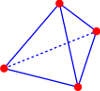

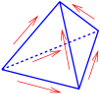
Nedelec’s tangentially-continuous \(H(curl)\)-conforming edge elements:

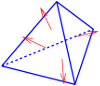
Raviart-Thomas normally-continuous \(H(div)\)-conforming face elements:

Discontinuous \(L_2\) elements:

These vector-valued spaces allow to represent physical quantities which are either normally or tangentially continuous.

The finite element spaces are related by the de Rham complex:

\[\begin{split}\DeclareMathOperator{\Grad}{grad} \DeclareMathOperator{\Curl}{curl} \DeclareMathOperator{\Div}{div} \begin{array}{ccccccc} H^1 & \stackrel{\Grad}{\longrightarrow} & H(\Curl) & \stackrel{\Curl}{\longrightarrow} & H(\Div) & \stackrel{\Div}{\longrightarrow} & L^2 \\[8pt] \bigcup & & \bigcup & & \bigcup & & \bigcup \\[8pt] W_{h} & \stackrel{\Grad}{\longrightarrow} & V_{h } & \stackrel{\Curl}{\longrightarrow} & Q_{h} & \stackrel{\Div}{\longrightarrow} & S_{h} \: \\[3ex] \end{array}\end{split}\]

NGSolve supports these elements of arbitrary order, on all common element shapes (trigs, quads, tets, prisms, pyramids, hexes). Elements may be curved.

from ngsolve import *
from ngsolve.webgui import Draw

mesh = Mesh(unit_square.GenerateMesh(maxh=0.3))

Generate a higher order \(H^1\)-space. We first explore its different types of basis functions.

order=3
fes = H1(mesh, order=order)
gfu = GridFunction(fes)

The first basis functions are hat-functions, one per vertex. By setting the solution vector to a unit-vector, we may look at the individual basis functions:

gfu.vec[:] = 0
# vertex nr 17:
gfu.vec[17] = 1
Draw(gfu, min=0, max=1, deformation=True);

The next are edge-bubbles, where we have \((p-1)\) basis functions per edge. A NodeId object refers to a particular vertex, edge, face or cell node in the mesh. We can ask for the degrees of freedom on a node:

# basis functions on edge nr:
edge_dofs = fes.GetDofNrs(NodeId(EDGE,10))
print("edge_dofs =", edge_dofs)
gfu.vec[:] = 0
gfu.vec[edge_dofs[0]] = -1
Draw(gfu, order=3, min=-0.05, max=0.05, deformation=True);

Finally, we have \((p-1)(p-2)/2\) inner basis functions on every triangle:

trig_dofs = fes.GetDofNrs(NodeId(FACE,0))
print("trig_dofs = ", trig_dofs)
gfu.vec[:] = 0
gfu.vec[trig_dofs[0]] = 10
Draw(gfu, order=3, min=0, max=0.3, deformation=True);

The FESpace also maintains information about local dofs, interface dofs and wire-basket dofs for the BDDC preconditioner:

for i in range(fes.ndof):
    print (i,":", fes.CouplingType(i))

\(H(curl)\) finite element space

In NGSolve we use hierarchical high order finite element basis functions with node-wise exact sequences. The lowest order space \(W_{l.o}\) is the edge-element space:

\[\begin{split}\begin{array}{rcll} W_{hp} & = & W_{p=1} + \sum_E W_E + \sum_F W_F + \sum_C W_C & \subset H^1 \\[0.5em] V_{hp} & = & W_{l.o} + \sum_E V_E + \sum_F V_F + \sum_C V_C & \subset H(curl) \end{array}\end{split}\]

where the edge, face and cell blocks are compatible in the sense that

\[\nabla W_E = V_E, \quad \nabla W_F \subset V_F, \quad \nabla W_C \subset V_C\]

We obtain this by using gradients of \(H^1\) basis functions as \(H(curl)\) basis functions, and some more (see thesis Sabine Zaglmayr):

\[\begin{split}\begin{array}{rcl} V_E & = & \text{span} \{ \nabla \varphi_{E,i}^{H^1} \} \\ V_F & = & \text{span} \{ \nabla \varphi_{F,i}^{H^1} \cup \widetilde \varphi_{F,i}^{H(curl)} \} \\ V_C & = & \text{span} \{ \nabla \varphi_{C,i}^{H^1} \cup \widetilde \varphi_{C,i}^{H(curl)} \} \end{array}\end{split}\]

fes = HCurl(mesh, order=2)
uc = GridFunction(fes, name="uc")

edge_dofs = fes.GetDofNrs(NodeId(EDGE,10))
print ("edgedofs: ", edge_dofs)
uc.vec[:] = 0
uc.vec[edge_dofs[0]] = 1
Draw (uc, min=0, max=3, vectors = { "grid_size":30})
Draw (curl(uc), mesh, "curl", min=-25, max=25);

face_dofs = fes.GetDofNrs(NodeId(FACE,10))
print ("facedofs: ", face_dofs)
uc.vec[:] = 0
uc.vec[face_dofs[0]] = 1
Draw (uc, min=0, max=1, vectors = { "grid_size":30})
Draw (curl(uc), mesh, "curl", min=-1, max=1, order=3); # it's a gradient

\(H(div)\) finite element space

NGSolve provides Raviart-Thomas (RT) as well as Brezzi-Douglas-Marini (BDM) finite element spaces for H(div). We obtain the RT-version by setting RT=True, otherwise we get BDM.

fes = HDiv(mesh, order=2, RT=True)
ud = GridFunction(fes)
func = x*y*(x,y)
ud.Set (func)
Draw (ud, vectors = { "grid_size":30})
print ("interpolation error:", Integrate ((func-ud)**2, mesh))

The function spaces know their canonical derivatives. These operations are efficiently implemented by transformation from the reference element.

gfu.derivname, ud.derivname, uc.derivname

But there are additional options, like forming the element-wise gradient of H(div) finite element functions. We can query the available operators via

print ("H(div) operators: ", ud.Operators())

and access them via the Operator() method

Draw (grad(ud)[0,1], mesh, "gradud");