2.1.4 Element-wise BDDC Preconditioner#

The element-wise BDDC (Balancing Domain Decomposition preconditioner with Constraints) preconditioner in NGSolve is a good general purpose preconditioner that works well both in the shared memory parallel mode as well as in distributed memory mode. In this tutorial, we discuss this preconditioner, related built-in options, and customization from python.

Let us start with a simple description of the element-wise BDDC in the context of Lagrange finite element space \(V\). Here the BDDC preconditioner is constructed on an auxiliary space \(\widetilde{V}\) obtained by connecting only element vertices (leaving edge and face shape functions discontinuous). Although larger, the auxiliary space allows local elimination of edge and face variables. Hence an analogue of the original matrix \(A\) on this space, named \(\widetilde A\), is less expensive to invert. This inverse is used to construct a preconditioner for \(A\) as follows:

\[C_{BDDC}^{-1} = R {\,\widetilde{A}\,}^{-1}\, R^t\]

Here, \(R\) is the averaging operator for the discontinuous edge and face variables.

To construct a general purpose BDDC preconditioner, NGSolve generalizes this idea to all its finite element spaces by a classification of degrees of freedom. Dofs are classified into (condensable) LOCAL_DOFs that we saw in 1.4 and a remainder that includes these types:

WIREBASKET_DOF

INTERFACE_DOF

The original finite element space \(V\) is obtained by requiring conformity of both the above types of dofs, while the auxiliary space \(\widetilde{V}\) is obtained by requiring conformity of WIREBASKET_DOFs only.

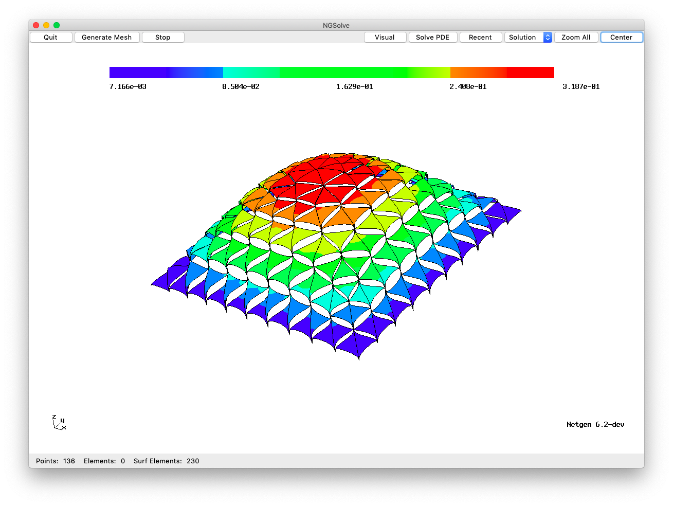
Here is a figure of a typical function in the default \(\widetilde{V}\) (and the code to generate this is at the end of this tutorial) when \(V\) is the Lagrange space:

title

[ ]:

from ngsolve import *
from ngsolve.webgui import Draw
from ngsolve.la import EigenValues_Preconditioner
SetHeapSize(100*1000*1000)

[ ]:

mesh = Mesh(unit_cube.GenerateMesh(maxh=0.5))
# mesh = Mesh(unit_square.GenerateMesh(maxh=0.5))

Built-in options#

Let us define a simple function to study how the spectrum of the preconditioned matrix changes with various options.

Effect of condensation#

[ ]:

def TestPreconditioner (p, condense=False, **args):
    fes = H1(mesh, order=p, **args)
    u,v = fes.TnT()
    a = BilinearForm(fes, eliminate_internal=condense)
    a += grad(u)*grad(v)*dx + u*v*dx
    c = Preconditioner(a, "bddc")
    a.Assemble()
    return EigenValues_Preconditioner(a.mat, c.mat)

[ ]:

lams = TestPreconditioner(5)
print (lams[0:3], "...\n", lams[-3:])

Here is the effect of static condensation on the BDDC preconditioner.

[ ]:

lams = TestPreconditioner(5, condense=True)
print (lams[0:3], "...\n", lams[-3:])

Tuning the auxiliary space#

Next, let us study the effect of a few built-in flags for finite element spaces that are useful for tweaking the behavior of the BDDC preconditioner. The effect of these flags varies in two (2D) and three dimensions (3D), e.g.,

wb_fulledges=True: This option keeps all edge-dofs conforming (i.e. they are marked WIREBASKET_DOFs). This option is only meaningful in 3D. If used in 2D, the preconditioner becomes a direct solver.
wb_withedges=True: This option keeps only the first edge-dof conforming (i.e., the first edge-dof is marked WIREBASKET_DOF and the remaining edge-dofs are marked INTERFACE_DOFs).

The complete situation is a bit more complex due to the fact these options can take the three values True, False, or Undefined, the two options can be combined, and the space dimension can be 2 or 3. The default value of these flags in NGSolve is Undefined. Here is a table with the summary of the effect of these options:

wb_fulledges	wb_withedges	2D	3D
True	any value	all	all
False/Undefined	Undefined	none	first
False/Undefined	False	none	none
False/Undefined	True	first	first

An entry \(X \in\) {all, none, first} of the last two columns is to be read as follows: \(X\) of the edge-dofs is(are) WIREBASKET_DOF(s).

Here is an example of the effect of one of these flag values.

[ ]:

lams = TestPreconditioner(5, condense=True,
                          wb_withedges=False)
print (lams[0:3], "...\n", lams[-3:])

Clearly, when moving from the default case (where the first of the edge dofs are wire basket dofs) to the case (where none of the edge dofs are wire basket dofs), the conditioning became less favorable.

Customize#

From within python, we can change the types of degrees of freedom of finite element spaces, thus affecting the behavior of the BDDC preconditioner.

To depart from the default and commit the first two edge dofs to wire basket, we perform the next steps:

[ ]:

fes = H1(mesh, order=10)
u,v = fes.TnT()

for ed in mesh.edges:
    dofs = fes.GetDofNrs(ed)
    for d in dofs:
        fes.SetCouplingType(d, COUPLING_TYPE.INTERFACE_DOF)

    # Set the first two edge dofs to be conforming
    fes.SetCouplingType(dofs[0], COUPLING_TYPE.WIREBASKET_DOF)
    fes.SetCouplingType(dofs[1], COUPLING_TYPE.WIREBASKET_DOF)

a = BilinearForm(fes, eliminate_internal=True)
a += grad(u)*grad(v)*dx + u*v*dx
c = Preconditioner(a, "bddc")
a.Assemble()

lams=EigenValues_Preconditioner(a.mat, c.mat)
max(lams)/min(lams)

This is a slight improvement from the default.

[ ]:

lams = TestPreconditioner (10, condense=True)
max(lams)/min(lams)

Combine BDDC with AMG for large problems#

The coarse inverse \({\,\widetilde{A}\,}^{-1}\) of BDDC is expensive on fine meshes. Using the option coarsetype=h1amg flag, we can ask BDDC to replace \({\,\widetilde{A}\,}^{-1}\) by an Algebraic MultiGrid (AMG) preconditioner. Since NGSolve’s h1amg is well-suited

for the lowest order Lagrange space, we use the option wb_withedges=False to ensure that \(\widetilde{A}\) is made solely with vertex unknowns.

[ ]:

p = 5
mesh = Mesh(unit_cube.GenerateMesh(maxh=0.05))
fes = H1(mesh, order=p, dirichlet="left|bottom|back",
         wb_withedges=False)
print("NDOF = ", fes.ndof)
u,v = fes.TnT()
a = BilinearForm(fes)
a += grad(u)*grad(v)*dx
f = LinearForm(fes)
f += v*dx

with TaskManager():
    pre = Preconditioner(a, "bddc", coarsetype="h1amg")
    a.Assemble()
    f.Assemble()

    gfu = GridFunction(fes)
    solvers.CG(mat=a.mat, rhs=f.vec, sol=gfu.vec,
               pre=pre, maxsteps=500)
Draw(gfu)

Postscript#

By popular demand, here is the code to draw the figure found at the beginning of this tutorial:

[ ]:

from netgen.geom2d import unit_square
mesh = Mesh(unit_square.GenerateMesh(maxh=0.1))
fes_ho = Discontinuous(H1(mesh, order=10))
fes_lo = H1(mesh, order=1, dirichlet=".*")
fes_lam = Discontinuous(H1(mesh, order=1))
fes = fes_ho*fes_lo*fes_lam
uho, ulo, lam = fes.TrialFunction()

a = BilinearForm(fes)
a += Variation(0.5 * grad(uho)*grad(uho)*dx
               - 1*uho*dx
               + (uho-ulo)*lam*dx(element_vb=BBND))
gfu = GridFunction(fes)
solvers.Newton(a=a, u=gfu)
Draw(gfu.components[0],deformation=True, settings={"camera": {"transformations": [{"type": "rotateX", "angle": -45}]}})